Welcome back for another year at Texas Tech. Below are links to the lecture notes for the topics we will be covering. There are also several links to other websites in the right-hand column of this page, to provide additional information.
Introductory Material (from 2015)
Preliminary Data-Analysis Issues
Review of ANOVA
MANOVA
Logistic Regression
Discriminant-Function Analysis
Log-Linear Modeling
Cluster Analysis
Multidimensional Scaling
Brief Overview of Advanced Topics (HLM, Missing Data, and Big Data)

Quantitative Methods III (Human Development & Family Studies 6364) at Texas Tech University
Saturday, August 27, 2016
Friday, November 27, 2015
Brief Overview of Advanced Topics: HLM, Missing Data, Big Data
Given that this was my first time teaching this course (Fall 2015), I could only guess as to how much time each topic would take to cover. As it turned out, we ran out of time to cover three topics, so I wanted to provide brief overviews of them.
Hierarchical Linear Modeling (HLM; also known as Multilevel Modeling). Updated Nov. 18, 2016. When participants are naturally organized in a hierarchical structure (e.g., students within classes, classes within schools), HLM is a suitable statistical approach. The researcher can study dynamics at both a more micro level (in the classroom) and more macro level (at the school).
For example, an elementary school may have 20 classrooms, each with 30 students (total N = 600). One approach would be to analyze relations among your variables of interest (e.g., students' academic efficacy, work habits, and grades) simply within your 600-student sample, not taking into account who each student's teacher is (an undifferentiated sample). However, statistical research (as well as several popular movies, such as this, this, and this) suggest that particular teachers can have an impact on students.
A variation on this approach would be to use the 600-student sample, adding a series of 19 dummy variables (a dummy variable for each teacher's name, e.g., "Smith," "Jones," etc., with one teacher omitted as a reference category) to indicate if a student had (scored as 1) or did not have (scored as 0) a particular teacher (dummy-variable refresher). Doing so will reveal relationships between variables (e.g., efficacy, work habits) in the 600 students, controlling for which teacher students had.
Yet another approach would be to average all the variables within each class, creating a dataset with an N of 20 (i.e., each class would be a case). Each class would have variables such as average student efficacy, average student work habits, and average student grade. In doing so, however, one commits the well-known ecological fallacy. The recent 2016 U.S. presidential election provides an example:
The need for a better analytic technique sets the stage for HLM. Here's an introductory video by Mark Tranmer (we'll start at the 10:00 point). Before watching the video, here are some important concepts to know:
Apparala, M. L., Reifman, A., & Munsch, J. (2003). Cross-national comparison of attitudes toward fathers' and mothers' participation in household tasks and childcare. Sex Roles, 48, 189-203.
Here's a link to the United Nations' Gender Empowerment Measure, which was a country-level predictor of citizens' attitudes toward couple egalitarianism in doing household tasks and childcare.
Missing Data. Nearly all datasets will have missing data, whether through participants declining to answer certain questions, accidentally overlooking items, or other reasons. Increasingly sophisticated techniques for dealing with missing data have been developed, but researchers must be careful that they're using appropriate methods. A couple of excellent overview articles on handling missing data are the following:
Acock, A. C. (2005). Working with missing values. Journal of Marriage and Family, 67, 1012–1028.
Schlomer, G. L., Bauman, S., & Card, N. A (2010). Best practices for missing data management in counseling psychology. Journal of Counseling Psychology, 57, 1-10
Also see additional resources in the links section to the right.
When one hears the term "mean substitution," it is important to distinguish between two possible meanings.
Big Data. The amount of capturable data people generate is truly mind-boggling, from commerce, health care, law enforcement, sports, and other domains. We will watch a brief video (see links section to the right) listing numerous examples. The study of Big Data (also known as "Data Mining") applies statistical techniques such as correlation and cluster analysis to discern patterns in the data and make predictions.
Among the many books appearing on the topic of Big Data, I would recommend Supercrunchers (by Ian Ayres) on business applications, The Victory Lab (by Sasha Issenberg) on political campaigns, and three books pertaining to baseball: Moneyball (by Michael Lewis) on the Oakland Athletics; The Extra 2% (by Jonah Keri) on the Tampa Bay Rays; and Big Data Baseball (by Travis Sawchik) on the Pittsburgh Pirates. These three teams play in relatively small cities by Major League Baseball standards and thus bring in less local-television revenue than the big-city teams. Therefore, teams such as Oakland, Tampa Bay, and Pittsburgh must use statistical techniques to (a) discover "deceptively good" players, whose skills are not well-known to other teams and who can thus be paid non-exorbitant salaries, and (b) identify effective strategies that other teams aren't using (yet). The Pirates' signature strategy, now copied by other teams, is the defensive shift, using statistical "spray charts" unique to each batter.
To end the course, here's one final song...
Big Data
Lyrics by Alan Reifman
May be sung to the tune of “Green Earrings” (Fagen/Becker for Steely Dan)
Sales, patterns,
Companies try,
Running equations,
To predict, what we’ll buy,
Big data,
Lots of numbers,
Floating in, the cloud,
For computers,
To analyze, now,
We know, how,
Sports, owners,
Wanting to win,
Seeking, advantage,
In the numbers, it’s no sin,
Big data,
Lots of numbers,
Floating in, the cloud,
For computers,
To analyze, now,
We know, how
Instrumentals/solos
Big data,
Lots of numbers,
Floating in, the cloud,
For computers,
To analyze, now,
We know, how
Instrumentals/solos
Hierarchical Linear Modeling (HLM; also known as Multilevel Modeling). Updated Nov. 18, 2016. When participants are naturally organized in a hierarchical structure (e.g., students within classes, classes within schools), HLM is a suitable statistical approach. The researcher can study dynamics at both a more micro level (in the classroom) and more macro level (at the school).
For example, an elementary school may have 20 classrooms, each with 30 students (total N = 600). One approach would be to analyze relations among your variables of interest (e.g., students' academic efficacy, work habits, and grades) simply within your 600-student sample, not taking into account who each student's teacher is (an undifferentiated sample). However, statistical research (as well as several popular movies, such as this, this, and this) suggest that particular teachers can have an impact on students.
A variation on this approach would be to use the 600-student sample, adding a series of 19 dummy variables (a dummy variable for each teacher's name, e.g., "Smith," "Jones," etc., with one teacher omitted as a reference category) to indicate if a student had (scored as 1) or did not have (scored as 0) a particular teacher (dummy-variable refresher). Doing so will reveal relationships between variables (e.g., efficacy, work habits) in the 600 students, controlling for which teacher students had.
Yet another approach would be to average all the variables within each class, creating a dataset with an N of 20 (i.e., each class would be a case). Each class would have variables such as average student efficacy, average student work habits, and average student grade. In doing so, however, one commits the well-known ecological fallacy. The recent 2016 U.S. presidential election provides an example:
- At the state level, six of the eight states with the largest African-American populations (as a percent of the state's total population) went Republican (this figure counts the District of Columbia as a state). Before we conclude that African-American voters strongly support the Republicans and Donald Trump, however, we should note that...
- At the individual level, national exit polls estimate that 88% of Black voters went for the Democrat, Hillary Clinton.
The need for a better analytic technique sets the stage for HLM. Here's an introductory video by Mark Tranmer (we'll start at the 10:00 point). Before watching the video, here are some important concepts to know:
- Intercept (essentially, the mean of a dependent variable y, when all predictors x are set to zero) and slope (relationship between x and y) of a line (click here for review).
- Fixed vs. random effects (summary).
- Individual- vs. group-level variables. Variables such as age and gender describe properties of an individual (e.g., 11-year-old girl, 9-year-old boy). Variables such as age of school buildings (mentioned in the video) and number of books in the library are characteristics of the school itself and hence, school- or group-level . Finally, individual person characteristics are sometimes averaged or otherwise aggregated to create a group-level variable (e.g., schools' percentages of students on free or reduced-cost meals, as an indicator of economic status). Whether a specific student receives a free/reduced-cost meal at school is an individual characteristic, but when portrayed as an average or percentage for the school, it becomes a group (school) characteristic. We might call these "derived" or "constructed" group-level variables as they're assembled from individual-level data, as opposed to being inherently school/group-level (like building age).
Apparala, M. L., Reifman, A., & Munsch, J. (2003). Cross-national comparison of attitudes toward fathers' and mothers' participation in household tasks and childcare. Sex Roles, 48, 189-203.
Here's a link to the United Nations' Gender Empowerment Measure, which was a country-level predictor of citizens' attitudes toward couple egalitarianism in doing household tasks and childcare.
Missing Data. Nearly all datasets will have missing data, whether through participants declining to answer certain questions, accidentally overlooking items, or other reasons. Increasingly sophisticated techniques for dealing with missing data have been developed, but researchers must be careful that they're using appropriate methods. A couple of excellent overview articles on handling missing data are the following:
Acock, A. C. (2005). Working with missing values. Journal of Marriage and Family, 67, 1012–1028.
Schlomer, G. L., Bauman, S., & Card, N. A (2010). Best practices for missing data management in counseling psychology. Journal of Counseling Psychology, 57, 1-10
Also see additional resources in the links section to the right.
When one hears the term "mean substitution," it is important to distinguish between two possible meanings.
- One involves filling in a participant's missing value on a variable with the mean for the sample on the same variable (i.e., sample-mean substitution). This approach appears to be widely discouraged.
- A second meaning involves a participant lacking data on a small number of items that are part of a multiple-item instrument (e.g., someone who answered only eight items on a 10-item self-esteem scale). In this case, it seems acceptable to let the mean of the answered items (that respondent's personal mean) stand in for what the mean of all the items on the instrument would have yielded had no answers been omitted. Essentially, one is assuming that the respondent would have answered the same way on the items left blank that he/she did on the completed items. I personally use a two-thirds rule for personal-mean substitution (e.g., if there were nine items on the scale, I would require at least six of the items to be answered; if not, the respondent would receive a "system-missing" value on the scale). See on this website where it says, "Allow for missing values."
Big Data. The amount of capturable data people generate is truly mind-boggling, from commerce, health care, law enforcement, sports, and other domains. We will watch a brief video (see links section to the right) listing numerous examples. The study of Big Data (also known as "Data Mining") applies statistical techniques such as correlation and cluster analysis to discern patterns in the data and make predictions.
Among the many books appearing on the topic of Big Data, I would recommend Supercrunchers (by Ian Ayres) on business applications, The Victory Lab (by Sasha Issenberg) on political campaigns, and three books pertaining to baseball: Moneyball (by Michael Lewis) on the Oakland Athletics; The Extra 2% (by Jonah Keri) on the Tampa Bay Rays; and Big Data Baseball (by Travis Sawchik) on the Pittsburgh Pirates. These three teams play in relatively small cities by Major League Baseball standards and thus bring in less local-television revenue than the big-city teams. Therefore, teams such as Oakland, Tampa Bay, and Pittsburgh must use statistical techniques to (a) discover "deceptively good" players, whose skills are not well-known to other teams and who can thus be paid non-exorbitant salaries, and (b) identify effective strategies that other teams aren't using (yet). The Pirates' signature strategy, now copied by other teams, is the defensive shift, using statistical "spray charts" unique to each batter.
To end the course, here's one final song...
Big Data
Lyrics by Alan Reifman
May be sung to the tune of “Green Earrings” (Fagen/Becker for Steely Dan)
Sales, patterns,
Companies try,
Running equations,
To predict, what we’ll buy,
Big data,
Lots of numbers,
Floating in, the cloud,
For computers,
To analyze, now,
We know, how,
Sports, owners,
Wanting to win,
Seeking, advantage,
In the numbers, it’s no sin,
Big data,
Lots of numbers,
Floating in, the cloud,
For computers,
To analyze, now,
We know, how
Instrumentals/solos
Big data,
Lots of numbers,
Floating in, the cloud,
For computers,
To analyze, now,
We know, how
Instrumentals/solos
Tuesday, November 17, 2015
Multidimensional Scaling
Updated November 23, 2015
Multidimensional Scaling (MDS) is a descriptive technique, to look for underlying dimensions or structure behind a set of objects. For a given set of objects, the similarity or dissimilarity between each pair must first be determined. This MDS overview document presents different ways of operationalizing similarity/dissimilarity. One ends up with a visual diagram, where more-similar objects end up physically close to each other. As with other techniques we've learned this semester (e.g., log-linear models, cluster analysis), there is no "official" way to determine which solution, of different possible ones, to accept. MDS provides different guidelines for how many dimensions to accept, one of which is the "stress" value (p. 13 of linked article).
The input to MDS in SPSS is either a similarity matrix (e.g., how similar is Object A to Object B? how similar is A to C? how similar is B to C?) or a dissimilarity/distance matrix. Zeroes are placed along the diagonal of the matrix, as it is not meaningful to talk about how similar A is to A, B is to B, etc.
A video on running MDS in SPSS can be accessed via the links column to the right. Once you select your visual solution, you get to name the dimensions, based on where the objects appear in the graph. The video illustrates the use of one particular MDS program called PROXSCAL, in which the numerical values in the input matrix can either represent similarities (i.e., higher numbers = greater similarity) or distances (i.e., higher numbers = greater dissimilarities).
However, the SPSS version we have in our computer lab does not provide access to PROXSCAL (not easily, at least) and only makes a program called ALSCAL readily available. In ALSCAL, higher numbers in the input matrix are read only as distances.
This is presumably where our initial analysis in last Thursday's class went awry. In trying to map the dimensions underlying our Texas Tech Human Development and Family Studies faculty members' research interests, we used the number of times each pair of faculty members had been co-authors on the same article as the measure of similarity. A high number of co-authorships would thus signify that the two faculty members in question had similar research interests. However, ALSCAL treats high numbers as indicative of greater distance (which I failed to catch at the time), thus messing up our analysis.
Once the numbers in the matrix are reverse-scored, so that a high number of co-authorships between a pair of faculty is converted to a low number for distance, then the MDS graph becomes more understandable. Below is an annotated screen-capture from SPSS, on which you can click to enlarge. (The graph does not show some of our newer faculty members, who would not have had much opportunity yet to publish with their faculty colleagues, or some of our faculty members who publish primarily with graduate students or with faculty from outside Texas Tech.)

The stress values shown in the output are somewhere between good and fair, according to the overview document linked above.

And now, our song for this topic...
Multidimensional Scaling is Fun
Lyrics by Alan Reifman
May be sung to the tune of “Minuano (Six Eight)” (Metheny/Mays)
YouTube video of performance here.
Multidimensional scaling, is fun,
Multidimensional scaling, is fun, to run, yeah,
Measure the objects’ similarities,
Or you can enter, as disparities, yes you can,
Multidimensional scaling, is fun,
SPSS is one place, that it’s done,
Submit your matrix in, and a spatial map, will come out,
Multidimensional scaling, is fun,
Multidimensional scaling, is fun,
Multidimensional scaling, is fun, to run, yeah,
Aim for a stress value, below point-ten,
Or you’ll have to run, your model again, yes you will,
Multidimensional scaling, is fun,
ALSCAL is one version, that you can run,
Submit your matrix in, and a spatial map, will come out,
Multidimensional scaling, is fun,
(Guitar improvisation 1:39-3:38, then piano and percussion interlude 3:38-4:55)
Multidimensional scaling, is fun,
Multidimensional scaling, is fun, to run, yeah,
Measure the objects’ similarities,
Or you can enter, as disparities, yes you can,
Multidimensional scaling, is fun,
SPSS is one place, that it’s done,
Submit your matrix in, and a spatial map, will come out,
Multidimensional scaling, is fun,
Multidimensional scaling, is fun,
Multidimensional scaling, is fun, to run, yeah,
Aim for a stress value, below point-ten,
Or you’ll have to run, your model again, yes you will,
Multidimensional scaling, is fun,
PROXSCAL’s another version, you can run,
Submit your matrix in, and a spatial map, will come out,
Multidimensional scaling, is fun,
Yes it’s fun,
Yes it’s fun,
Yes it’s fun,
Let it run!
Tuesday, October 27, 2015
Cluster Analysis
Updated November 2, 2015
Cluster analysis is a descriptive tool to find interesting subgroups of participants in your data. It's somewhat analogous to sorting one's disposables at a recycling center: glass items go in one bin, clear plastic in another, opaque plastic in another, etc. The items in any one bin are similar to each other, but the contents of one bin are different from those in another bin.
Typically, the researcher will have a domain of interest, such as political attitudes, dining preferences, or goals in life. Several items (perhaps 5-10) in the relevant domain will be submitted to cluster analysis. Participants who answer similarly to the items will be grouped into the same cluster, so that each cluster will be internally homogeneous, but different clusters will be different from each other.
Here's a very conceptual illustration, using the music-preference items from the 1993 General Social Survey (click image to enlarge)...

The color-coding shows the beginning stage of dividing the respondents into clusters:
Though the general approach of cluster analysis is relatively straightforward, actual implementation is fairly technical. The are two main approaches -- k-means/iterative and hierarchical -- that will be discussed. Key to both methods is determining similarity (or conversely, distance) between cases. The more similar cases are to each other, the more likely they will end up in the same cluster.
k-means/Iterative -- This approach is spatial, very much like discriminant analysis. One must specify the number (k) of clusters one seeks in an analysis, each one having a centroid (again like discriminant analysis). Cases are sorted into groups (clusters), based on which centroid they're closest to. The analysis goes through an iterative (repetitive) process of relocating centroids and determining data-points' distance from them, until the solution doesn't change anymore, as I illustrate in the following graphic.

Methods for locating initial centroids are discussed here. Naftali Harris has an excellent interactive webpage called "Visualizing K-Means Clustering," which illustrates many of the above steps.
There are different criteria for distance, such as single-linkage, average-linkage, etc. (See slide 17 of this slideshow.)
Hierarchical -- This approach uses a dendrogram (tree-diagram), which looks like a sports-tournament bracket college-basketball fans fill out every March with their predictions. As Rapkin and Luke (1993) describe:
Agglomerative hierarchical algorithms start with all cases as separate entities. Cases are combined (agglomerated) in sequence, so that those closest together are placed into the same cluster early in the hierarchy. As the analysis proceeds, small clusters of cases combine to form continually larger and more heterogeneous clusters, until all cases are joined into a single cluster (p. 267).
A particular kind of hierarchical clustering technique is Ward's method, which is said to be conducive to balanced cluster sizes (i.e., each cluster having a roughly equal number of cases, rather than some huge and some tiny clusters).
An "oldie, but goody" introductory article on cluster analysis is the following. The software descriptions are obviously out-of-date, but the general overview is excellent. Of particular value, in my view, is the set of recommendations for determining the number of clusters to retain (pp. 268-270).
Rapkin, B., & Luke, D. (1993). Cluster analysis in community research: Epistemology and practice. American Journal of Community Psychology, 21, 247-277.
An article that illustrates the use of cluster analysis, including how to characterize and name the clusters, is:
Schrick, B., Sharp, E. A., Zvonkovic, A., & Reifman, A. (2012). Never let them see you sweat: Silencing and striving to appear perfect among US college women. Sex Roles, 67, 591-604.
One final issue is the stability of cluster solutions. Even within k-means/iterative methods alone, or hierarchical methods alone, there are many ways to implement cluster analysis. To ensure your cluster solution is not merely the peculiar result of one method, you can use more than one method with the same dataset (e.g., one k-means/iterative method and one hierarchical method). You can save the assigned-memberships in SPSS for both methods and then run a cross-tab of these memberships to verify that the same people would end up grouped together (for the most part) in the various clusters.
As an analogy, think of the "Sorting Hat" in the Harry Potter series, which assigns new students at Hogwarts School into one of the four houses (clusters). Imagine that Headmaster Dumbledore decides to run a quality check on the Sorting Hat, bringing in another hat to independently conduct a second sorting of the kids into houses, so it can be seen if the two hats arrive at similar solutions. In the following hypothetical set of results, the two hats indeed arrive at largely similar solutions, although there are a few disagreements.

And, of course, we have a song...
Run Me Off a Cluster
Lyrics by Alan Reifman
May be sung to the tune of “Hey, Soul Sister” (Monahan/Bjørklund/Lind)
O-K, what we’ll learn, today,
What we’ll learn, today,
Are there, groupings?
Of participants, with the same things?
We use, formulas, for distance,
Compactness, is our insistence,
Within each cluster,
But different sets,
Should be as, far apart as,
Distance gets, oh yeah,
So pick an operation,
There are two main, realizations,
Of clustering techniques,
Hey there, Buster,
Run me off, a cluster...ing, analysis,
A synthesis, to help group our participants,
Hey there, Buster,
Run me off, a cluster…ing, analysis,
Tonight,
Hey, hey,
Hey, hey, hey, hey, hey,
Hey, hey, hey, hey, hey,
A dendrogram,
Is at the heart of,
Hierarchy-based plans, oh yeah,
Each case starts out, as a cluster,
Into pairs, they all will muster,
Then form, larger groups,
In number space,
Clusters and k-mean spots,
Will take their place, oh year,
Testing maps by, iteration,
Till it hits, the final station,
Then we’ll all take, a vacation,
Hey there, Buster,
Run me off, a cluster...ing, analysis,
A synthesis, to help group our participants,
Hey there, Buster,
Run me off, a cluster…ing, analysis,
Tonight,
There’s no official way,
To decide, how many clusters stay,
There are some criteria,
To take consideration of,
Your clusters, need interpretation,
On items, from their derivation,
I hope you find, some cool combinations,
Hey there, Buster,
Run me off, a cluster...ing, analysis,
A synthesis, to help group our participants,
Hey there, Buster,
Run me off, a cluster…ing, analysis,
Tonight,
Hey, hey,
Hey, hey, hey, hey, hey,
Hey, hey, hey, hey, hey,
Tonight,
Hey, hey,
Hey, hey, hey, hey, hey,
Hey, hey, hey, hey, hey,
Tonight...
Cluster analysis is a descriptive tool to find interesting subgroups of participants in your data. It's somewhat analogous to sorting one's disposables at a recycling center: glass items go in one bin, clear plastic in another, opaque plastic in another, etc. The items in any one bin are similar to each other, but the contents of one bin are different from those in another bin.
Typically, the researcher will have a domain of interest, such as political attitudes, dining preferences, or goals in life. Several items (perhaps 5-10) in the relevant domain will be submitted to cluster analysis. Participants who answer similarly to the items will be grouped into the same cluster, so that each cluster will be internally homogeneous, but different clusters will be different from each other.
Here's a very conceptual illustration, using the music-preference items from the 1993 General Social Survey (click image to enlarge)...

The color-coding shows the beginning stage of dividing the respondents into clusters:
- People whose responses are shaded orange tend to like big band, blues, Broadway musicals, and jazz, and dislike rap and heavy metal.
- Those in yellow really like jazz, and are moderately favorable toward country, blues, and rap.
- Those in green appear to dislike music generally!
Though the general approach of cluster analysis is relatively straightforward, actual implementation is fairly technical. The are two main approaches -- k-means/iterative and hierarchical -- that will be discussed. Key to both methods is determining similarity (or conversely, distance) between cases. The more similar cases are to each other, the more likely they will end up in the same cluster.
k-means/Iterative -- This approach is spatial, very much like discriminant analysis. One must specify the number (k) of clusters one seeks in an analysis, each one having a centroid (again like discriminant analysis). Cases are sorted into groups (clusters), based on which centroid they're closest to. The analysis goes through an iterative (repetitive) process of relocating centroids and determining data-points' distance from them, until the solution doesn't change anymore, as I illustrate in the following graphic.

Methods for locating initial centroids are discussed here. Naftali Harris has an excellent interactive webpage called "Visualizing K-Means Clustering," which illustrates many of the above steps.
There are different criteria for distance, such as single-linkage, average-linkage, etc. (See slide 17 of this slideshow.)
Hierarchical -- This approach uses a dendrogram (tree-diagram), which looks like a sports-tournament bracket college-basketball fans fill out every March with their predictions. As Rapkin and Luke (1993) describe:
Agglomerative hierarchical algorithms start with all cases as separate entities. Cases are combined (agglomerated) in sequence, so that those closest together are placed into the same cluster early in the hierarchy. As the analysis proceeds, small clusters of cases combine to form continually larger and more heterogeneous clusters, until all cases are joined into a single cluster (p. 267).
A particular kind of hierarchical clustering technique is Ward's method, which is said to be conducive to balanced cluster sizes (i.e., each cluster having a roughly equal number of cases, rather than some huge and some tiny clusters).
An "oldie, but goody" introductory article on cluster analysis is the following. The software descriptions are obviously out-of-date, but the general overview is excellent. Of particular value, in my view, is the set of recommendations for determining the number of clusters to retain (pp. 268-270).
Rapkin, B., & Luke, D. (1993). Cluster analysis in community research: Epistemology and practice. American Journal of Community Psychology, 21, 247-277.
An article that illustrates the use of cluster analysis, including how to characterize and name the clusters, is:
Schrick, B., Sharp, E. A., Zvonkovic, A., & Reifman, A. (2012). Never let them see you sweat: Silencing and striving to appear perfect among US college women. Sex Roles, 67, 591-604.
One final issue is the stability of cluster solutions. Even within k-means/iterative methods alone, or hierarchical methods alone, there are many ways to implement cluster analysis. To ensure your cluster solution is not merely the peculiar result of one method, you can use more than one method with the same dataset (e.g., one k-means/iterative method and one hierarchical method). You can save the assigned-memberships in SPSS for both methods and then run a cross-tab of these memberships to verify that the same people would end up grouped together (for the most part) in the various clusters.
As an analogy, think of the "Sorting Hat" in the Harry Potter series, which assigns new students at Hogwarts School into one of the four houses (clusters). Imagine that Headmaster Dumbledore decides to run a quality check on the Sorting Hat, bringing in another hat to independently conduct a second sorting of the kids into houses, so it can be seen if the two hats arrive at similar solutions. In the following hypothetical set of results, the two hats indeed arrive at largely similar solutions, although there are a few disagreements.

And, of course, we have a song...
Run Me Off a Cluster
Lyrics by Alan Reifman
May be sung to the tune of “Hey, Soul Sister” (Monahan/Bjørklund/Lind)
O-K, what we’ll learn, today,
What we’ll learn, today,
Are there, groupings?
Of participants, with the same things?
We use, formulas, for distance,
Compactness, is our insistence,
Within each cluster,
But different sets,
Should be as, far apart as,
Distance gets, oh yeah,
So pick an operation,
There are two main, realizations,
Of clustering techniques,
Hey there, Buster,
Run me off, a cluster...ing, analysis,
A synthesis, to help group our participants,
Hey there, Buster,
Run me off, a cluster…ing, analysis,
Tonight,
Hey, hey,
Hey, hey, hey, hey, hey,
Hey, hey, hey, hey, hey,
A dendrogram,
Is at the heart of,
Hierarchy-based plans, oh yeah,
Each case starts out, as a cluster,
Into pairs, they all will muster,
Then form, larger groups,
In number space,
Clusters and k-mean spots,
Will take their place, oh year,
Testing maps by, iteration,
Till it hits, the final station,
Then we’ll all take, a vacation,
Hey there, Buster,
Run me off, a cluster...ing, analysis,
A synthesis, to help group our participants,
Hey there, Buster,
Run me off, a cluster…ing, analysis,
Tonight,
There’s no official way,
To decide, how many clusters stay,
There are some criteria,
To take consideration of,
Your clusters, need interpretation,
On items, from their derivation,
I hope you find, some cool combinations,
Hey there, Buster,
Run me off, a cluster...ing, analysis,
A synthesis, to help group our participants,
Hey there, Buster,
Run me off, a cluster…ing, analysis,
Tonight,
Hey, hey,
Hey, hey, hey, hey, hey,
Hey, hey, hey, hey, hey,
Tonight,
Hey, hey,
Hey, hey, hey, hey, hey,
Hey, hey, hey, hey, hey,
Tonight...
Wednesday, October 14, 2015
Log-Linear Modeling
Log-linear modeling, which is used when one has a set of entirely nominal/categorical variables, is an extension of the chi-square analysis for two nominal variables. As you'll recall, with chi-square analyses, we compare actual/observed frequencies of people within each cell, with expected frequencies. With log-linear modeling (LLM), one can analyze three, four, or more nominal variables in relationship to each other. The name comes from the fact that LLM use logarithms in the calculations (along with odds and odds ratios, like logistic regression).
Many sources state that with LLM there is no distinction between independent and dependent variables. I think it's still OK to think of IV's (predictors) in relation to a DV, however. In the example below (from the 1993 General Social Survey), the DV is political party identification (collapsed into Democratic [strong, weak], Republican [strong, weak], and Independent ["pure" Independent, Ind. Lean Dem., and Ind. Lean. Repub.]). Predictors are religious affiliation (collapsing everyone other than Protestant and Catholic into "All Other & None"); college degree (yes/no), and gender.
Variables are typically represented by their initial (P, R, C, and G in our example). Further, putting two or more letters together (with no comma) signifies relationships among the respective variables. By convention, one's starting (or baseline) model posits that the DV (in this case, party identification) is unrelated to the three predictors, but the predictors are allowed to relate to each other. The symbolism [P, RCG] describes the hypothesis that one's decision to self-identify as a Democrat, Republican, or Independent (and make one's voting decisions accordingly) is not influenced in any way by one's religious affiliation, attainment (or not) of a college degree, or gender. However, any relationships in the data between predictors are taken into account. Putting the three predictors together (RCG) also allows for three-way relationships or interactions, such as if Catholic females had a high rate of getting bachelor's degrees (which I have no idea if it's true). Three-way interaction terms (e.g., Religion X College X Gender) also include all two-way interactions (RC, RG, CG) contained within.
The orange column in the chart below shows us how many respondents actually appeared in each of the 36 cells representing combinations of political party (3) X religion (3) X college-degree (2) X gender (2).
The next column to the right shows us the expected frequencies generated by the [P, RCG] baseline model. We would not expect this model to do a great job of predicting cell frequencies, because it does not allow Party ID to be predicted by religion, college, or gender. Indeed, the expected frequencies under this model do not match the actual frequencies very well. I have highlighted in purple any cell in which the expected frequency comes within +/- 3 people of the actual frequency (the +/- 3 criterion is arbitrary; I just thought it gives a good feel for how well a given model does). The [P, RCG] model produces only 7 purple cells out of 36 possible. Each model also generates a chi-square value (use the likelihood-ratio version). As a reminder from previous stat classes, chi-square represents discrepancy (O-E) or "badness of fit," so a highly significant chi-square value for a given model signifies poor match to the actual frequencies. Significance levels for each model are indicated in the respective red boxes atop each column (***p < .001, **p < .01, *p < .05).
After running the baseline model and obtaining its chi-square value, we then move on to more complex models that add relationships or linkages between the predictors and DV. The second red column shows expected frequencies for the model [PR, RCG]. This model keeps the previous RCG combination, but now adds a relationship between party (P) and religious (R) affiliation. If there is some relationship between party and religion, such as Protestants being more likely than other religious groups to identify as a Republican, the addition of the PR term will result in a substantial improvement in the match between expected frequencies for this model and the actual frequencies. Indeed, the [PR, RCG] model produces 16 well-fitting (purple) cells, a much better performance than the previous model. (Adding linkages such as PR instead of just P will either improve the fit or leave it the same; it cannot harm fit.)

Let's step back a minute and consider all the elements in the [P, RCG] and [PR, RCG] models:
[P, RCG]: P, RCG, RC, RG, CG, R, C, G
[PR, RCG]: PR, P, RCG, RC, RG, CG, R, C, G
Notice that all the terms in the first model are included within the second model, but the second model has one additional term (PR). The technical term is that the first model is nested within the second. Nestedness is required to conduct some of the statistical comparisons we will discuss later.
If we look at the model [PC, RCG], we see that it contains:
PC, P, RCG, RC, RG, CG, R, C, G
The two models highlighted in yellow are not nested. To go from [PR, RCG] to [PC, RCG], you would have to delete the PR term (because the latter doesn't have PR) and add the PC term. When you have to both add and subtract, two models are not nested.
Let's return to discussing models that allow R, C, and/or G to relate to P. As noted above, adding more linkages will improve the fit between actual and expected frequencies. However, we want to add as few linkages as possible in order to keep the model as simple or parsimonious as possible.
The next model in the above chart is [PC, RCG], which allows college-degree status (but no other variables) predict party ID. There's not much extra bang (9 purple cells) for the buck (using PC instead of just P). The next model [PG, RCG], which specifies gender as the sole predictor of party ID, yields 11 purple cells. If you could only have one predictor relate to party ID, the choice would be religion (16 purple cells).
We're not so limited, however. We can allow two or even all three predictors to relate to party ID. The fifth red column presents [PRC, RCG], which allows religion, college-degree, and the two combined to predict party ID. Perhaps being a college-educated Catholic disproportionately is associated with identifying as a Democrat (again, I don't know if this is actually true). As with all the previous models, the RCG term allows all the predictors to relate to each other. As it turns out, [PRC, RCG] is the best model of all the ones tested, yielding 18 purple cells. The other two-predictor models, [PRG, RCG] and [PCG, RCG], don't do quite as well.
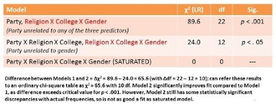
The final model, on the far right (spatially, not politically) is known as [PRCG]. It allows religion, college-degree, and gender -- individually and in combination -- to predict party ID. In this sense, it's a four-way interaction. As noted, a given interaction includes all lower-order terms, so [PRCG] also includes PRC, PRG, PCG, RCG, PR, PC, PG, RC, RG, RC, P, R, G, and G. Inclusion of all possible terms, as is the case here, is known as a saturated model. A saturated model will yield estimated frequencies that match perfectly the actual frequencies. It's no great accomplishment; it's a mathematical necessity. (Saturation and perfect fit also feature prominently in the next course in our statistical sequence, Structural Equation Modeling.)
Ideally, among the models tested, at least one non-saturated model will show a non-significant chi-square (badness of fit) on its own. That didn't happen in the present set of models, but the model I characterized above as the best [PRC, RCG] is "only" significant at p < .05, compared to p < .001 for all the other non-saturated models. Also, as shown in the following table, [PRC, RCG] fits significantly better than the baseline [P, RCG] by what is known as the delta chi-square test. Models must be nested within each other for such a test to be permissible. (For computing degrees of freedom, see Knoke & Burke, 1980, Log-Linear Models, Sage, pp. 36-37.)
When you tell SPSS to run the saturated model, it automatically gives you a supplemental backward-elimination analysis, which is described here. This is another way to help decide which model best approximates the actual frequencies.
My colleagues and I used log-linear modeling in one of our articles:
Fitzpatrick, J., Sharp, E. A., & Reifman, A. (2009). Midlife singles’ willingness to date partners with heterogeneous characteristics. Family Relations, 58 , 121–133.
Finally, we have a song:
Log-Linear Models
Lyrics by Alan Reifman
May be sung to the tune of “I Think We’re Alone Now” (Ritchie Cordell; performed by Tommy James and others)
Below, Dr. Reifman chats with Tommy James, who performed at the 2013 South Plains Fair and was kind enough to stick around and visit with fans and sign autographs. Dr. Reifman tells Tommy about how he (Dr. Reifman) has written statistical lyrics to Tommy's songs for teaching purposes.

Chi-square, two-way, is what we're used, to analyzing,
But, what if you've, say, three or four nominal variables?
Reading all the stat books that you can, seeking out what you can understand,
Trying to find techniques, specifically for, multi-way categorical data,
And you finally find a page, and there it says:
Log-linear models,
You try to re-create, the known frequencies,
Log-linear models,
You try to use as few, hypothesized links,
Each step of the way, you let it use associations,
You build an array, until the point of saturation,
Reading all the stat books that you can, seeking out what you can understand,
Trying to find techniques, specifically for, multi-way categorical data,
And you finally find a page, and there it says:
Log-linear models,
You try to re-create, the known frequencies,
Log-linear models,
You try to use as few, hypothesized links,
Many sources state that with LLM there is no distinction between independent and dependent variables. I think it's still OK to think of IV's (predictors) in relation to a DV, however. In the example below (from the 1993 General Social Survey), the DV is political party identification (collapsed into Democratic [strong, weak], Republican [strong, weak], and Independent ["pure" Independent, Ind. Lean Dem., and Ind. Lean. Repub.]). Predictors are religious affiliation (collapsing everyone other than Protestant and Catholic into "All Other & None"); college degree (yes/no), and gender.
Variables are typically represented by their initial (P, R, C, and G in our example). Further, putting two or more letters together (with no comma) signifies relationships among the respective variables. By convention, one's starting (or baseline) model posits that the DV (in this case, party identification) is unrelated to the three predictors, but the predictors are allowed to relate to each other. The symbolism [P, RCG] describes the hypothesis that one's decision to self-identify as a Democrat, Republican, or Independent (and make one's voting decisions accordingly) is not influenced in any way by one's religious affiliation, attainment (or not) of a college degree, or gender. However, any relationships in the data between predictors are taken into account. Putting the three predictors together (RCG) also allows for three-way relationships or interactions, such as if Catholic females had a high rate of getting bachelor's degrees (which I have no idea if it's true). Three-way interaction terms (e.g., Religion X College X Gender) also include all two-way interactions (RC, RG, CG) contained within.
The orange column in the chart below shows us how many respondents actually appeared in each of the 36 cells representing combinations of political party (3) X religion (3) X college-degree (2) X gender (2).
The next column to the right shows us the expected frequencies generated by the [P, RCG] baseline model. We would not expect this model to do a great job of predicting cell frequencies, because it does not allow Party ID to be predicted by religion, college, or gender. Indeed, the expected frequencies under this model do not match the actual frequencies very well. I have highlighted in purple any cell in which the expected frequency comes within +/- 3 people of the actual frequency (the +/- 3 criterion is arbitrary; I just thought it gives a good feel for how well a given model does). The [P, RCG] model produces only 7 purple cells out of 36 possible. Each model also generates a chi-square value (use the likelihood-ratio version). As a reminder from previous stat classes, chi-square represents discrepancy (O-E) or "badness of fit," so a highly significant chi-square value for a given model signifies poor match to the actual frequencies. Significance levels for each model are indicated in the respective red boxes atop each column (***p < .001, **p < .01, *p < .05).
After running the baseline model and obtaining its chi-square value, we then move on to more complex models that add relationships or linkages between the predictors and DV. The second red column shows expected frequencies for the model [PR, RCG]. This model keeps the previous RCG combination, but now adds a relationship between party (P) and religious (R) affiliation. If there is some relationship between party and religion, such as Protestants being more likely than other religious groups to identify as a Republican, the addition of the PR term will result in a substantial improvement in the match between expected frequencies for this model and the actual frequencies. Indeed, the [PR, RCG] model produces 16 well-fitting (purple) cells, a much better performance than the previous model. (Adding linkages such as PR instead of just P will either improve the fit or leave it the same; it cannot harm fit.)

Let's step back a minute and consider all the elements in the [P, RCG] and [PR, RCG] models:
[P, RCG]: P, RCG, RC, RG, CG, R, C, G
[PR, RCG]: PR, P, RCG, RC, RG, CG, R, C, G
Notice that all the terms in the first model are included within the second model, but the second model has one additional term (PR). The technical term is that the first model is nested within the second. Nestedness is required to conduct some of the statistical comparisons we will discuss later.
If we look at the model [PC, RCG], we see that it contains:
PC, P, RCG, RC, RG, CG, R, C, G
The two models highlighted in yellow are not nested. To go from [PR, RCG] to [PC, RCG], you would have to delete the PR term (because the latter doesn't have PR) and add the PC term. When you have to both add and subtract, two models are not nested.
Let's return to discussing models that allow R, C, and/or G to relate to P. As noted above, adding more linkages will improve the fit between actual and expected frequencies. However, we want to add as few linkages as possible in order to keep the model as simple or parsimonious as possible.
The next model in the above chart is [PC, RCG], which allows college-degree status (but no other variables) predict party ID. There's not much extra bang (9 purple cells) for the buck (using PC instead of just P). The next model [PG, RCG], which specifies gender as the sole predictor of party ID, yields 11 purple cells. If you could only have one predictor relate to party ID, the choice would be religion (16 purple cells).
We're not so limited, however. We can allow two or even all three predictors to relate to party ID. The fifth red column presents [PRC, RCG], which allows religion, college-degree, and the two combined to predict party ID. Perhaps being a college-educated Catholic disproportionately is associated with identifying as a Democrat (again, I don't know if this is actually true). As with all the previous models, the RCG term allows all the predictors to relate to each other. As it turns out, [PRC, RCG] is the best model of all the ones tested, yielding 18 purple cells. The other two-predictor models, [PRG, RCG] and [PCG, RCG], don't do quite as well.
The final model, on the far right (spatially, not politically) is known as [PRCG]. It allows religion, college-degree, and gender -- individually and in combination -- to predict party ID. In this sense, it's a four-way interaction. As noted, a given interaction includes all lower-order terms, so [PRCG] also includes PRC, PRG, PCG, RCG, PR, PC, PG, RC, RG, RC, P, R, G, and G. Inclusion of all possible terms, as is the case here, is known as a saturated model. A saturated model will yield estimated frequencies that match perfectly the actual frequencies. It's no great accomplishment; it's a mathematical necessity. (Saturation and perfect fit also feature prominently in the next course in our statistical sequence, Structural Equation Modeling.)
Ideally, among the models tested, at least one non-saturated model will show a non-significant chi-square (badness of fit) on its own. That didn't happen in the present set of models, but the model I characterized above as the best [PRC, RCG] is "only" significant at p < .05, compared to p < .001 for all the other non-saturated models. Also, as shown in the following table, [PRC, RCG] fits significantly better than the baseline [P, RCG] by what is known as the delta chi-square test. Models must be nested within each other for such a test to be permissible. (For computing degrees of freedom, see Knoke & Burke, 1980, Log-Linear Models, Sage, pp. 36-37.)

When you tell SPSS to run the saturated model, it automatically gives you a supplemental backward-elimination analysis, which is described here. This is another way to help decide which model best approximates the actual frequencies.
My colleagues and I used log-linear modeling in one of our articles:
Fitzpatrick, J., Sharp, E. A., & Reifman, A. (2009). Midlife singles’ willingness to date partners with heterogeneous characteristics. Family Relations, 58 , 121–133.
Finally, we have a song:
Log-Linear Models
Lyrics by Alan Reifman
May be sung to the tune of “I Think We’re Alone Now” (Ritchie Cordell; performed by Tommy James and others)
Below, Dr. Reifman chats with Tommy James, who performed at the 2013 South Plains Fair and was kind enough to stick around and visit with fans and sign autographs. Dr. Reifman tells Tommy about how he (Dr. Reifman) has written statistical lyrics to Tommy's songs for teaching purposes.
Chi-square, two-way, is what we're used, to analyzing,
But, what if you've, say, three or four nominal variables?
Reading all the stat books that you can, seeking out what you can understand,
Trying to find techniques, specifically for, multi-way categorical data,
And you finally find a page, and there it says:
Log-linear models,
You try to re-create, the known frequencies,
Log-linear models,
You try to use as few, hypothesized links,
Each step of the way, you let it use associations,
You build an array, until the point of saturation,
Reading all the stat books that you can, seeking out what you can understand,
Trying to find techniques, specifically for, multi-way categorical data,
And you finally find a page, and there it says:
Log-linear models,
You try to re-create, the known frequencies,
Log-linear models,
You try to use as few, hypothesized links,
Log-linear models,
You try to re-create, the known frequencies,
Log-linear models,
You try to use as few, hypothesized links,
Log-linear models,
You try to re-create, the known frequencies,
Log-linear models,
You try to use as few, hypothesized links,
You try to re-create, the known frequencies,
Log-linear models,
You try to use as few, hypothesized links,
Log-linear models,
You try to re-create, the known frequencies,
Log-linear models,
You try to use as few, hypothesized links,
Log-linear models,
You try to re-create, the known frequencies,
Log-linear models,
You try to use as few, hypothesized links,
You try to re-create, the known frequencies,
Log-linear models,
You try to use as few, hypothesized links,
Sunday, September 27, 2015
Discriminant Function Analysis
We've just finished logistic regression, which uses a set of variables to predict status on a two-category outcome, such as whether college students graduate or don't graduate. What if we wanted to make finer distinctions, say into three categories: graduated, dropped-out, and transferred to another school?
There is an extension of logistic regression, known as multinomial logistic regression, which uses a series of pairwise comparisons (e.g., dropped-out vs. graduates, transferred vs. graduates). See explanatory PowerPoint in the links section to the right.
Discriminant function analysis (DFA) allows you to put all three (or more) groups into one analysis. DFA uses spatial-mathematical principles to map out the three (or more) groups' spatial locations (with each group having a mean or "centroid") on a system of axes defined by the predictor variables. As a result, you get neat diagrams such as this, this, and this.
DFA, like statistical modeling in general, generates a somewhat oversimplified solution that is accurate for a large proportion of cases, but has some error. An example can be seen in this document (see Figure 4). Classification accuracy is one of the statistics one receives in DFA output.
(A solution that would be accurate for all cases might be popular, but wouldn't be useful. As Nate Silver writes in his book The Signal and The Noise, you would have "an overly specific solution to a general problem. This is overfitting, and it leads to worse predictions"; p. 163 )
The axes, known as canonical discriminant functions, are defined in the structure matrix, which shows correlations between your predictor variables and the functions. An example appears in this document dealing with classification of obsidian archaeological finds (see Figure 7-17 and Table 7-18). A warning: Archaeology is a career that often ends in ruins!
[The presence of groups and coefficients may remind you of MANOVA. According to lecture notes from Andrew Ainsworth, "MANOVA and discriminant function analysis are mathematically identical but are different in terms of emphasis. [Discriminant] is usually concerned with actually putting people into groups (classification) and testing how well (or how poorly) subjects are classified. Essentially, discrim is interested in exactly how the groups are differentiated not just that they are significantly different (as in MANOVA)."]
The following article illustrates a DFA with a mainstream HDFS topic:
Hazan, C., & Shaver, P. R. (1987). Romantic love conceptualized as an attachment process. Journal of Personality and Social Psychology, 52, 511-524.
Finally, this video, as well as this document, explain how to implement and interpret DFA in SPSS. And here's our latest song...
Discriminant!
Lyrics by Alan Reifman
May be sung to the tune of “Notorious” (LeBon/Rhodes/Taylor for Duran Duran)
Disc-disc-discriminant, discriminant!
Disc-disc-discriminant!
(Funky bass groove)
You’ve got multiple groups, all made from categories,
To predict membership, IV’s can tell their stories,
A technique, you can use,
It’s called discriminant -- the results are imminent,
You get an equation, for who belongs in the sets,
Number of functions, you subtract one, from sets,
To form the functions, you get the coefficients,
These weight the IV’s, to yield a composite score,
These scores determine, how it sorts the people,
That’s how, discriminant runs,
Disc-disc...
You can see in a graph, how all the groups are deployed,
Each group has a home base, which is known, as a “centroid,”
Weighted IV’s on axes, how you keep track -- it's just like, you're reading a map,
See how each group differs, from all the other ones there,
Number of functions, you subtract one, from sets,
To form the functions, you get the coefficients,
These weight the IV’s, to yield a composite score,
These scores determine, how it sorts the people,
That’s how, discriminant runs,
Disc-
Disc-disc...
(Brief interlude)
Discriminant,
Number of functions, you subtract one, from sets,
To form the functions, you get the coefficients,
These weight the IV’s, to yield a composite score,
These scores determine, how it sorts the people,
Number of functions, you subtract one, from sets,
To form the functions, you get the coefficients,
These weight the IV’s, to yield a composite score,
These scores determine, how it sorts the people,
That’s how, discriminant runs,
Disc-discriminant,
Disc-Disc,
That’s how, discriminant runs,
Disc-
Yeah, that’s how, discriminant runs,
Disc-Disc,
(Sax improvisation)
Yeah...That’s how, discriminant runs,
Disc-discriminant,
Disc-disc-discriminant...
There is an extension of logistic regression, known as multinomial logistic regression, which uses a series of pairwise comparisons (e.g., dropped-out vs. graduates, transferred vs. graduates). See explanatory PowerPoint in the links section to the right.
Discriminant function analysis (DFA) allows you to put all three (or more) groups into one analysis. DFA uses spatial-mathematical principles to map out the three (or more) groups' spatial locations (with each group having a mean or "centroid") on a system of axes defined by the predictor variables. As a result, you get neat diagrams such as this, this, and this.
DFA, like statistical modeling in general, generates a somewhat oversimplified solution that is accurate for a large proportion of cases, but has some error. An example can be seen in this document (see Figure 4). Classification accuracy is one of the statistics one receives in DFA output.
(A solution that would be accurate for all cases might be popular, but wouldn't be useful. As Nate Silver writes in his book The Signal and The Noise, you would have "an overly specific solution to a general problem. This is overfitting, and it leads to worse predictions"; p. 163 )
The axes, known as canonical discriminant functions, are defined in the structure matrix, which shows correlations between your predictor variables and the functions. An example appears in this document dealing with classification of obsidian archaeological finds (see Figure 7-17 and Table 7-18). A warning: Archaeology is a career that often ends in ruins!
[The presence of groups and coefficients may remind you of MANOVA. According to lecture notes from Andrew Ainsworth, "MANOVA and discriminant function analysis are mathematically identical but are different in terms of emphasis. [Discriminant] is usually concerned with actually putting people into groups (classification) and testing how well (or how poorly) subjects are classified. Essentially, discrim is interested in exactly how the groups are differentiated not just that they are significantly different (as in MANOVA)."]
The following article illustrates a DFA with a mainstream HDFS topic:
Hazan, C., & Shaver, P. R. (1987). Romantic love conceptualized as an attachment process. Journal of Personality and Social Psychology, 52, 511-524.
Finally, this video, as well as this document, explain how to implement and interpret DFA in SPSS. And here's our latest song...
Discriminant!
Lyrics by Alan Reifman
May be sung to the tune of “Notorious” (LeBon/Rhodes/Taylor for Duran Duran)
Disc-disc-discriminant, discriminant!
Disc-disc-discriminant!
(Funky bass groove)
You’ve got multiple groups, all made from categories,
To predict membership, IV’s can tell their stories,
A technique, you can use,
It’s called discriminant -- the results are imminent,
You get an equation, for who belongs in the sets,
Number of functions, you subtract one, from sets,
To form the functions, you get the coefficients,
These weight the IV’s, to yield a composite score,
These scores determine, how it sorts the people,
That’s how, discriminant runs,
Disc-disc...
You can see in a graph, how all the groups are deployed,
Each group has a home base, which is known, as a “centroid,”
Weighted IV’s on axes, how you keep track -- it's just like, you're reading a map,
See how each group differs, from all the other ones there,
Number of functions, you subtract one, from sets,
To form the functions, you get the coefficients,
These weight the IV’s, to yield a composite score,
These scores determine, how it sorts the people,
That’s how, discriminant runs,
Disc-
Disc-disc...
(Brief interlude)
Discriminant,
Number of functions, you subtract one, from sets,
To form the functions, you get the coefficients,
These weight the IV’s, to yield a composite score,
These scores determine, how it sorts the people,
Number of functions, you subtract one, from sets,
To form the functions, you get the coefficients,
These weight the IV’s, to yield a composite score,
These scores determine, how it sorts the people,
That’s how, discriminant runs,
Disc-discriminant,
Disc-Disc,
That’s how, discriminant runs,
Disc-
Yeah, that’s how, discriminant runs,
Disc-Disc,
(Sax improvisation)
Yeah...That’s how, discriminant runs,
Disc-discriminant,
Disc-disc-discriminant,
That’s how, discriminant runs,Disc-discriminant,
Disc-disc-discriminant...
Monday, September 21, 2015
Logistic Regression
This week, we'll review ordinary regression (for quantitative dependent variables such as dollars of earnings or GPA at college graduation) and then begin coverage of logistic regression (for dichotomous DV's). Both kinds of regression allow all kinds of predictor variables (quantitative and categorical/dummy variables). Logistic regression involves mathematical elements that may be unfamiliar to some, so we'll go over everything step-by-step.
The example we'll work through is a bit unconventional, but one with a Lubbock connection. Typically, our cases are persons. In this example, however, the cases are songs -- Paul McCartney songs. McCartney, of course, was a member of the Beatles (1960-1970), considered by many the greatest rock-and-roll band of all-time. After the Beatles broke up, McCartney led a new group called Wings (1971-1981), before performing as a solo act. For many years after the Beatles' break-up, he declined to perform his old Beatles songs, but finally resumed doing so in 1989.
Given that McCartney has a catalog of close to 500 songs (excluding ones written entirely or primarily by other members of the Beatles), the question was which songs he would play in his 2014 Lubbock concert. I obtained lists of songs written by McCartney here and here, and a playlist from his Lubbock concert here. Any given song could be played or not played in Lubbock -- a dichotomous dependent variable. The independent variable was whether McCartney wrote the song while with the Beatles or post-Beatles (for Wings or as a solo performer).
This analysis could be done as a 2 (Beatles/post-Beatles era) X 2 (yes/no played in Lubbock) chi-square, but we'll examine it via logistic regression for illustrative purposes. Note that logistic-regression analyses usually would have multiple predictor variables, not just one. The null hypothesis would be that any given non-Beatles song would have the same probability of being played as any given Beatles song. What I really expected, however, was that Beatles songs would have a higher probability of being played than non-Beatles songs.
Following are some PowerPoint slides I made to explain logistic regression, using the McCartney concert example. We'll start out with some simple cross-tabular frequencies and introduction of the concept of odds.

Next are some mathematical formulations of logistic regression (as opposed to the general linear model that informs ordinary regression) and part of the SPSS output from the McCartney example.

(Here's a reference documenting that any number raised to the zero power is one; technically, any non-zero number raised to the zero power is one.)
Note that odds ratios work not only when moving from a score of zero to a score of one on a predictor variable (as in the song example). The prior odds are multiplied by the same factor (the OR) whether moving from zero to one, one to two, two to three, etc.
The last slide is a chart showing general guidelines for interpreting logistic-regression B coefficients and odds ratios. Logistic regression is usually done with unstandardized predictor variables.

The book Applied Logistic Regression by Hosmer, Lemeshow, and Sturdivant is a good resource. We'll also look at some of the materials in the links column to the right and some articles that used logistic regression, and run some example analyses in SPSS.
--------------------------------------------------------------------------------------------------------------------------
One last thing I like to do when working with complex multivariate statistics is run a simpler analysis as an analogue, to understand what's going on. Hopefully, the results from the actual multivariate analysis and the simplified analogue will be similar. A basic cross-tab can be used to simulate what a logistic regression is doing. Consider the following example from the General Social Survey (GSS) 1993 practice data set in SPSS. The dichotomous DV is whether a respondent had obtained a college degree or not, and the predictor variables were age, mother's highest educational level, father's highest educational level, one's own number of children, and one's attitude toward Broadway musicals (high value = strong dislike).
The logistic-regression equation, shown at the top of the following graphic, reveals that father's education (an ordinal variable ranging from less than a high-school diploma [0] to graduate-school degree [4]) had an odds ratio (OR) of 1.53. This tells us that, controlling for all other predictors, each one-unit increment on father's level of educational attainment would raise the respondent's odds of obtaining a college degree by a multiplicative factor of 1.53.

One might expect, therefore, that if we run a cross-tab of father's education (rows) by own degree status (columns), the odds of the respondent having a college degree will increase by 1.53 times, as father's education goes up a level. This is not the case, as shown in the graphic. When the father's educational attainment was less than a high-school diploma, the grown child's odds of having a college degree were .142. When father's education was one level higher, namely a high-school diploma (scored as 1), the grown child's odds of having a college degree became .376. The value .376 is 2.65 times greater than the previous odds of .142, not 1.53 times greater.
A couple of things can be said at this point. First, the cross-tab utilizes only two variables, father's education and grown child's college-degree status; none of the other predictor variables are controlled for. Second, it is an obvious oversimplification to say that an individual's odds of having a college degree should increase by a uniform multiplier (in this case, 1.53) for each increment in father's educational attainment. In reality, the odds might go up by somewhat more than 1.53 between some levels of father's education and by somewhat less than 1.53 between other levels of father's education. However, as long as the 1.53 factor matches the step-by-step multipliers from the cross-tabs reasonably well, it simplifies things greatly to have a single value for the multiplier. (We will discuss this idea of accuracy vs. simplicity later in the course.)
One question that might have occurred to some of you is whether the multiplier values in the cross-tab (2.65, 2.09, etc.) might match logistic-regression results more accurately if we ran a logistic regression with father's education as the only predictor. In fact, averaging the four blue multipliers in the graphic matches very closely with the OR from such an analysis. Whether such a match will generally occur or just occurred this time by chance, I don't know.
--------------------------------------------------------------------------------------------------------------------------
Finally, we have a song. I actually wrote it back in 2007, for a guest lecture I gave in QM III.
e Raised to the B Power
Lyrics by Alan Reifman
(May be sung to the tune of “Rikki Don’t Lose That Number,” Becker/Fagen for Steely Dan)
(SLOW) Running logistic regression...
For a dichotomous outcome, it’s designed,
Predictor variables can be, any kind,
But what will be your key result?
e raised to the B power,
That’s what gives you the, Odds Ratio,
This is something important, you must know,
e raised to the B power,
When an IV rises one,
DV odds multiply by O.R.,
It’s so much fun!
Will faculty make tenure, yes or no?
Say the O.R. for pubs, is 1.5,
For each new article, then, we multiply,
By this determined ratio,
e raised to the B power,
That’s what gives you the, Odds Ratio,
This is something important, you must know,
e raised to the B power,
When an IV rises one,
DV odds multiply by O.R.,
And then you’re done...
(Guitar solo)
--------------------------------------------------------------------------------------------------------------------------
One last thing I like to do when working with complex multivariate statistics is run a simpler analysis as an analogue, to understand what's going on. Hopefully, the results from the actual multivariate analysis and the simplified analogue will be similar. A basic cross-tab can be used to simulate what a logistic regression is doing. Consider the following example from the General Social Survey (GSS) 1993 practice data set in SPSS. The dichotomous DV is whether a respondent had obtained a college degree or not, and the predictor variables were age, mother's highest educational level, father's highest educational level, one's own number of children, and one's attitude toward Broadway musicals (high value = strong dislike).
The logistic-regression equation, shown at the top of the following graphic, reveals that father's education (an ordinal variable ranging from less than a high-school diploma [0] to graduate-school degree [4]) had an odds ratio (OR) of 1.53. This tells us that, controlling for all other predictors, each one-unit increment on father's level of educational attainment would raise the respondent's odds of obtaining a college degree by a multiplicative factor of 1.53.

One might expect, therefore, that if we run a cross-tab of father's education (rows) by own degree status (columns), the odds of the respondent having a college degree will increase by 1.53 times, as father's education goes up a level. This is not the case, as shown in the graphic. When the father's educational attainment was less than a high-school diploma, the grown child's odds of having a college degree were .142. When father's education was one level higher, namely a high-school diploma (scored as 1), the grown child's odds of having a college degree became .376. The value .376 is 2.65 times greater than the previous odds of .142, not 1.53 times greater.
A couple of things can be said at this point. First, the cross-tab utilizes only two variables, father's education and grown child's college-degree status; none of the other predictor variables are controlled for. Second, it is an obvious oversimplification to say that an individual's odds of having a college degree should increase by a uniform multiplier (in this case, 1.53) for each increment in father's educational attainment. In reality, the odds might go up by somewhat more than 1.53 between some levels of father's education and by somewhat less than 1.53 between other levels of father's education. However, as long as the 1.53 factor matches the step-by-step multipliers from the cross-tabs reasonably well, it simplifies things greatly to have a single value for the multiplier. (We will discuss this idea of accuracy vs. simplicity later in the course.)
--------------------------------------------------------------------------------------------------------------------------
e Raised to the B Power
Lyrics by Alan Reifman
(May be sung to the tune of “Rikki Don’t Lose That Number,” Becker/Fagen for Steely Dan)
(SLOW) Running logistic regression...
For a dichotomous outcome, it’s designed,
Predictor variables can be, any kind,
But what will be your key result?
e raised to the B power,
That’s what gives you the, Odds Ratio,
This is something important, you must know,
e raised to the B power,
When an IV rises one,
DV odds multiply by O.R.,
It’s so much fun!
Will faculty make tenure, yes or no?
Say the O.R. for pubs, is 1.5,
For each new article, then, we multiply,
By this determined ratio,
e raised to the B power,
That’s what gives you the, Odds Ratio,
This is something important, you must know,
e raised to the B power,
When an IV rises one,
DV odds multiply by O.R.,
And then you’re done...
(Guitar solo)
Subscribe to:
Posts (Atom)